DisCVR Built-in Databases

DisCVR tool has three virus k-mers (k=22) databases which are built into the DisCVR.jar:

1. Human Hemorrhagic virus dataset (hemorrhagic dataset)
2. Human Respiratory virus dataset (respiratory dataset)
3. Human Pathogenic viruses dataset (pathogenic dataset)

The hemorrhagic and respiratory datasets consist of a list of selected circulating viruses. The pathogenic datatset consist of a list of all human pathogenic viruses identified as biological agents by the Health and Safety Executive (HSE) in the UK available at: http://www.hse.gov.uk/pubns/misc208.pdf

Both the hemorrhagic and respiratory datasets overlap with the HSE database but are smaller in size and therefore are faster to use in classification. Moreover, each dataset has a list of viral reference genomes that is associated with the viruses in the database. The reference genomes are used in the validation stage of DisCVR. Information about the viruses in the databases can be obtained from the Database icon on the menu bar from the DisCVR GUI. The information includes the virus rank on the taxonomy tree, the number of sequences used in the database build to represent it, and the accession number of its reference genome. Segmented viruses have their reference genome accession number listed in decreasing order of the segment size. The accession numbers of the reference genomes are linked to their webpages on the NCBI, which can be viewed by clicking on the reference genome accession.

DisCVR Classification

The DisCVR GUI can be used to carry out a single sample classification. To launch the DisCVR GUI, either double click on DisCVR.jar, or open a command prompt and type the following commands:

cd full/path/to/DisCVR folder
java –jar full/path/to/DisCVR.jar

Once DisCVR is launched, there are 4 panels in the graphical interface:

1. Progress Bar: shows the progression of the classification process.
2. Input Sources: allows the user to choose the sample file and a k-mers database for classification.
3. Classification Results: shows the classification output in three sub-panels.
4. Progress Information: updates the user about classification output.

To start a classification process, the user needs to first select the sample file they wish to investigate. Currently, DisCVR supports .fasta, .fa, .fastq, and .fq formats. It allows for the selection of one file hence, for paired-end files, it is recommended to concatenate both files. The second step is to choose the database for the classification. The default setting is to select one of the three built-in databases. This sets the k-mer size to 22 and removes all sample k-mers with entropy ≤ 2.5. On the other hand, if the user chooses to use a customised database for the classification, then the box next to the Customised Database label must be checked. The fields for this selection are then activated for the user to upload the customised database file, which MUST be in the customisedDB folder that is in the same path as DisCVR.jar. The k-mer size for the classification is extracted from the database name and the threshold to filter out low-entropy k-mers from the sample should be entered in its corresponding field. The entropy threshold should be the same value used in the build of the customised database which is recommended to be in the range of [0, 3.0]. If the users choose not to specify a value for the entropy threshold then the default value of 2.5 is displayed in the field and used in the classification.

Once, the database library is selected, the user clicks the classify button to start the classification process.

There are 4 stages in the classification process and the progress bar is updated after the completion of each stage. Messages in relation to the output of each stage are displayed in the progress information panel. This includes the number of reads in the sample, the number of distinct k-mers and their total counts in the database and the sample file, the number of sample k-mers after removing single copies and low entropy k-mers, and the number of classified k-mers and their total counts. The final message shows the number of viruses with classified *k*mers found in the sample and the time taken to finish the classification process. Figure 1 shows screenshots of the sample classification process using the DisCVR GUI.

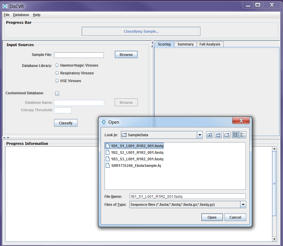
Figure2a: Screenshots of a sample classification process using DisCVR GUI. First the sample file is uploaded

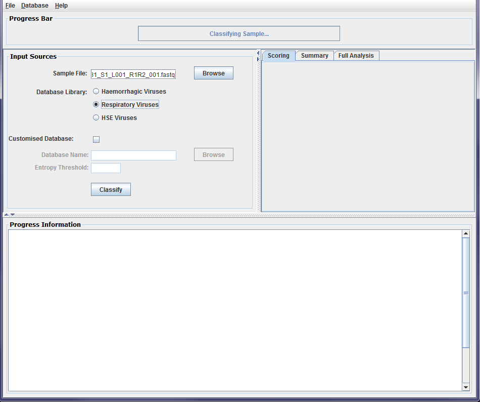
Figure2b: Screenshots of a sample classification process using DisCVR GUI. The k-mers database is then selected from the DisCVR database library

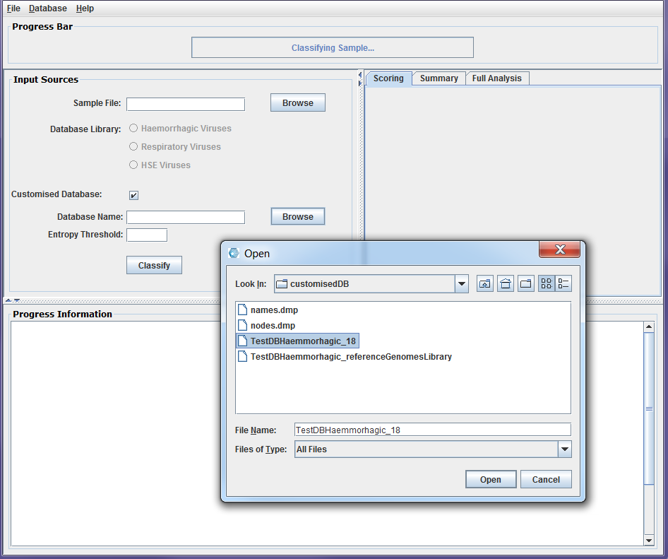
Figure2b: Screenshots of a sample classification process using DisCVR GUI. The k-mers database is then selected from the user customised database*

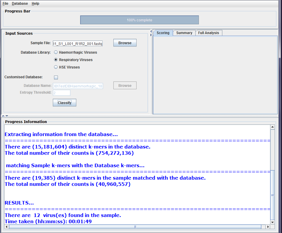
Figure2b: Screenshots of a sample classification process using DisCVR GUI. The classification results are displayed

Classification Output

At the end of the classification process, the progress information panel states the number of viruses with matched k-mers to the database. Detailed information about the classification results are displayed on the centre panel.

The classification results panel consists of three sub-panels: Scoring, Summary, and Full Analysis. Once the classification is completed, a bar chart showing up the top three viruses is displayed on the scoring panel. These are the viruses with the most number of classified distinct k-mers found in the sample. The chart shows for each virus, the number of distinct k-mers that are specific to the virus as well as the number of shared k-mers with other viruses in the sample, which are referred to as non-specific k-mers. The Summary panel gives a list of the viruses found in the sample along with their number of specific and non-specific distinct k-mers. The Full Analysis panel shows a table with taxonomic and detailed information about the viruses with classified k-mers from the sample. The results are shown in the table such that the first row shows the virus with the highest number of k-mers found in the sample. However, the users can click on any column heading to sort out the results in the table according to the information in the column. The full analysis table consists of 8 columns:

1. Virus Name: the scientific name for the virus taking from the NCBI names.dmp file.
2. Taxa ID: the taxonomy identification for the virus in the NCBI taxonomy tree.
3. Virus Rank: the rank of the virus according to the NCBI nodes.dmp file.

4. Total counts of k-mers in DB: the total counts of k-mers that represent the virus in DisCVR’s database.

5. No. of distinct Classified k-mers: the number of distinct k-mers that represent the virus in the sample after removing single copies and low entropy k-mers and matched with the k-mers database.

6. (%) of distinct Classified k-mers: the percentage of distinct classified k-mers that represent the virus in the sample.

7. Total counts of Classified k-mers: the total number of k-mers that represent the virus in the sample; some distinct k-mers can occur in the reads multiple times.

8. (%) of total classified k-mers: the percentage of the total number of k-mers that represent the virus in the sample’s total number of k-mers.

The table can be saved as .csv file from the File icon on the GUI tool bar. Figure 2 shows screenshots of the classification results sub-panels.

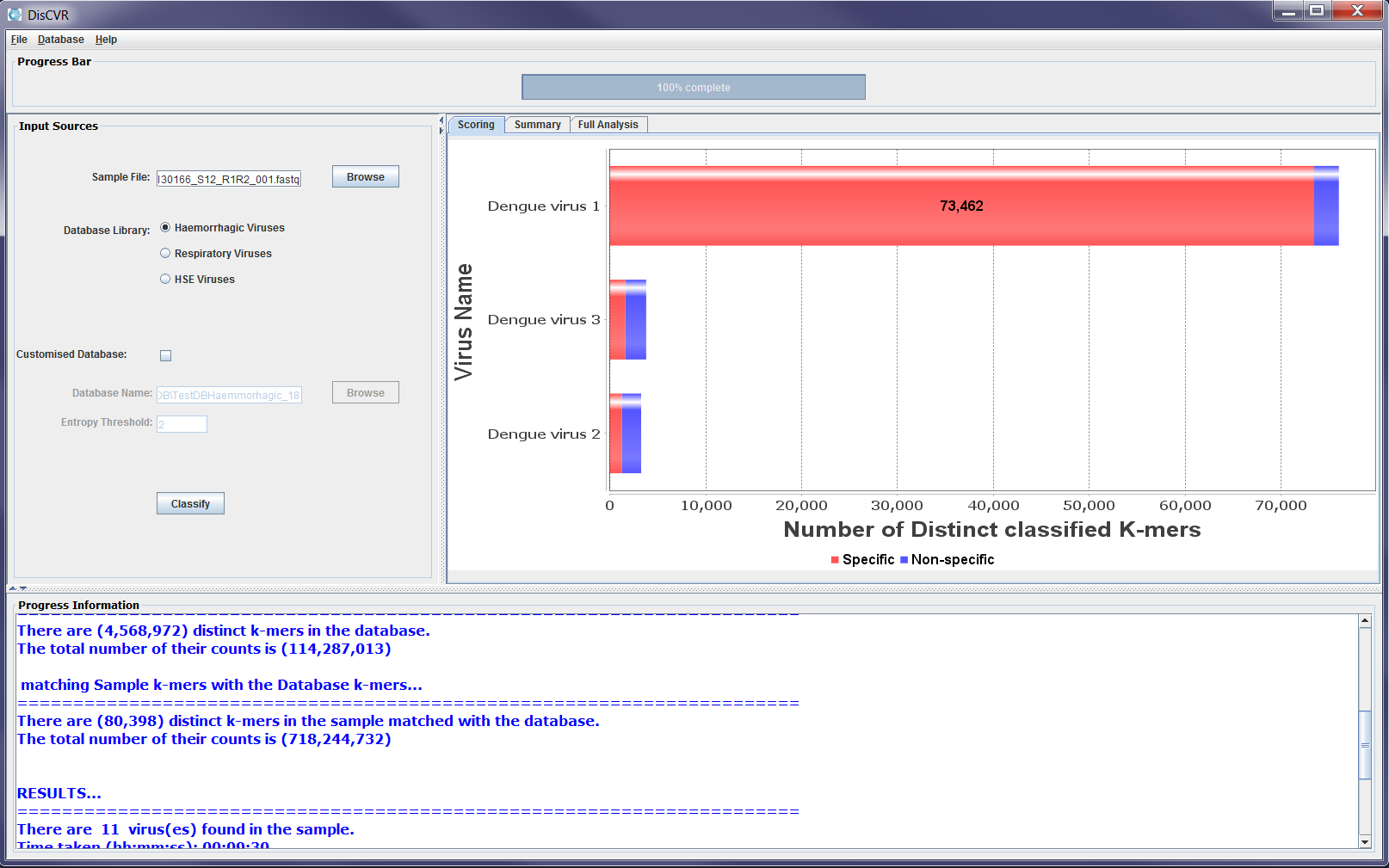
Figure3a: Screenshots showing sample classification output on the results sub-panels. The scoring panel shows the three viruses with the highest number of matched k-mers

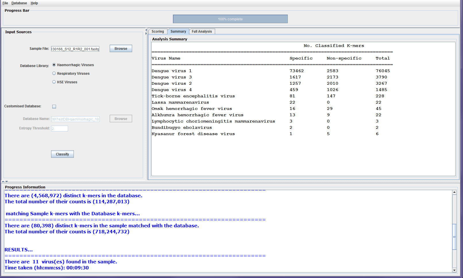
Figure3b: Screenshots showing sample classification output on the results sub-panels. The summary panel

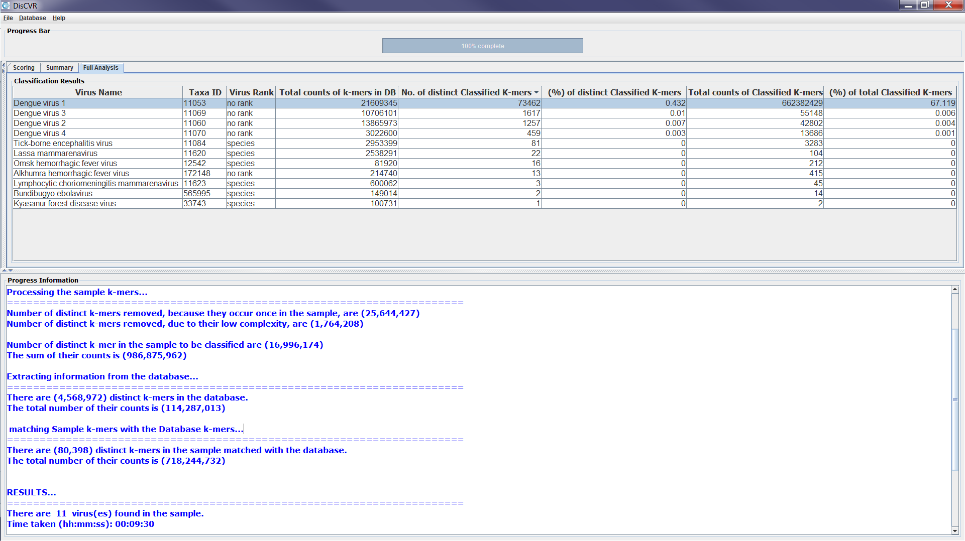
Figure3c: Screenshots showing sample classification output on the results sub-panels. The full analysis panel with detailed information about the viruses found in the sample